
Predicting Salaries for Job Postings
Chenxu Wen, chenxu.wen.math@gmail.com
Table of contents
Introduction and Import
In this report, I performed descriptive and predictive analysis on a data set about job postings. The goal is to understand the factors affecting job salaries and to predict future salaries.
Data Import
The job posting datasets are imported into Python. The first five rows of data are shown.
# import libraries
import numpy as np
import pandas as pd
from matplotlib import pyplot as plt
%matplotlib inline
import seaborn as sns
import pandas as pd
# import in the training data set
train = pd.read_csv("train_features_2013-03-07.csv", low_memory=False)
# only drop rows that are all NA:
train = train.dropna(how='all')

# read the target variable - salary
target = pd.read_csv("train_salaries_2013-03-07.csv")

# read the test data
test = pd.read_csv("test_features_2013-03-07.csv")
# take a look at the first 5 rows of train data
train.head()
| jobId | companyId | jobType | degree | major | industry | yearsExperience | milesFromMetropolis | |
|---|---|---|---|---|---|---|---|---|
| 0 | JOB1362684407687 | COMP37 | CFO | MASTERS | MATH | HEALTH | 10 | 83 |
| 1 | JOB1362684407688 | COMP19 | CEO | HIGH_SCHOOL | NONE | WEB | 3 | 73 |
| 2 | JOB1362684407689 | COMP52 | VICE_PRESIDENT | DOCTORAL | PHYSICS | HEALTH | 10 | 38 |
| 3 | JOB1362684407690 | COMP38 | MANAGER | DOCTORAL | CHEMISTRY | AUTO | 8 | 17 |
| 4 | JOB1362684407691 | COMP7 | VICE_PRESIDENT | BACHELORS | PHYSICS | FINANCE | 8 | 16 |
# take a look at the first 5 rows of test data
test.head()
| jobId | companyId | jobType | degree | major | industry | yearsExperience | milesFromMetropolis | |
|---|---|---|---|---|---|---|---|---|
| 0 | JOB1362685407687 | COMP33 | MANAGER | HIGH_SCHOOL | NONE | HEALTH | 22 | 73 |
| 1 | JOB1362685407688 | COMP13 | JUNIOR | NONE | NONE | AUTO | 20 | 47 |
| 2 | JOB1362685407689 | COMP10 | CTO | MASTERS | BIOLOGY | HEALTH | 17 | 9 |
| 3 | JOB1362685407690 | COMP21 | MANAGER | HIGH_SCHOOL | NONE | OIL | 14 | 96 |
| 4 | JOB1362685407691 | COMP36 | JUNIOR | DOCTORAL | BIOLOGY | OIL | 10 | 44 |
# take a look at the first 5 rows of target data
target.head()
| jobId | salary | |
|---|---|---|
| 0 | JOB1362684407687 | 130 |
| 1 | JOB1362684407688 | 101 |
| 2 | JOB1362684407689 | 137 |
| 3 | JOB1362684407690 | 142 |
| 4 | JOB1362684407691 | 163 |
The top 5 rows in the train, test, and target data are shown above. From the table, we can see that there are 8 columns in the data, including job ID, company ID, job type, degree required, major required, industry, years of experience required, and distance from metropolis. The outcome value is saved in the target variable.
Sanity Checks
Once the data is imported, let’s perform a few sanity checks on the data, including:
- missingness - are there missing values in the data?
- duplicates - are there duplicates in the data?
- observation and feature order - do observations and feature appear in the same order?
- outliers - are there outliers in both the predictors and the outcome?
- categorical levels - do train and test data have the same factor levels?
Missing Data Check
# check the number of entries and data type for each variable
train.info()
<class 'pandas.core.frame.DataFrame'>
Int64Index: 1000000 entries, 0 to 999999
Data columns (total 8 columns):
jobId                  1000000 non-null object
companyId              1000000 non-null object
jobType                1000000 non-null object
degree                 1000000 non-null object
major                  1000000 non-null object
industry               1000000 non-null object
yearsExperience        1000000 non-null int64
milesFromMetropolis    1000000 non-null int64
dtypes: int64(2), object(6)
memory usage: 68.7+ MB
# check the number of entries and data type for each variable
test.info()
<class 'pandas.core.frame.DataFrame'>
RangeIndex: 1000000 entries, 0 to 999999
Data columns (total 8 columns):
jobId                  1000000 non-null object
companyId              1000000 non-null object
jobType                1000000 non-null object
degree                 1000000 non-null object
major                  1000000 non-null object
industry               1000000 non-null object
yearsExperience        1000000 non-null int64
milesFromMetropolis    1000000 non-null int64
dtypes: int64(2), object(6)
memory usage: 61.0+ MB
# check the number of entries and data type for each variable
target.info()
<class 'pandas.core.frame.DataFrame'>
RangeIndex: 1000000 entries, 0 to 999999
Data columns (total 2 columns):
jobId     1000000 non-null object
salary    1000000 non-null int64
dtypes: int64(1), object(1)
memory usage: 15.3+ MB
Information on each variable in the train and test data is shown above. From the information, we can see that this is a relatively large data set with 1 million observations, with no missing data.
Duplicates Check
## check duplicates in train data
print('Are all observations in train unique?')
print(len(train.jobId.unique()) == train.shape[0])
Are all observations in train unique?
True
## check duplicates in test data
print('Are all observations in test unique?')
print(len(test.jobId.unique()) == test.shape[0])
Are all observations in test unique?
True
# now check if there's any overlap between train and test in terms of job postings
print('The number of job IDs in the test dataset that did appear in the train dataset:')
print(len ( set(test['jobId']).intersection( train['jobId'] ) ) )

print('The number of job IDs in the train dataset that did appear in the test dataset:')
print(len ( set(train['jobId']).intersection( test['jobId'] ) ) )
The number of job IDs in the test dataset that did appear in the train dataset:
0
The number of job IDs in the train dataset that did appear in the test dataset:
0
It’s good news that there’s no overlap between train and test, because otherwise there’d be leakage in the model training.
Observation and Feature Order Check
Here let’s check if the observations appear in the same order in the train data and target data. If not, we’ll need to sort the target to match the train dataset.
# let's check if the jobID appear in the same order in train and in target
# if not, we'll need to sort the target to match the train dataset
sum(train.jobId == target.jobId) == train.shape[0]
True
Now, let’s check if the features appear in the same order in the train and test data. If not, we’ll need to sort the test data to match the train data.
sum(train.columns == test.columns) == train.shape[1]
True
Outliers Check
Now we know that there’s no overlap between train and test observations, and that the features appear in the same order in train and test, we can safely concatenate the two DataFrames together for further analysis. Otherwise, we need to use the merge the two datasets.
# for the purpose of less typing, let's concat the train and test data
data = pd.concat([train, test], keys=['train','test'])
# get a quick description of numeric values in the data
data.describe()
| yearsExperience | milesFromMetropolis | |
|---|---|---|
| count | 2.000000e+06 | 2.000000e+06 |
| mean | 1.199724e+01 | 4.952784e+01 |
| std | 7.212785e+00 | 2.888372e+01 |
| min | 0.000000e+00 | 0.000000e+00 |
| 25% | 6.000000e+00 | 2.500000e+01 |
| 50% | 1.200000e+01 | 5.000000e+01 |
| 75% | 1.800000e+01 | 7.500000e+01 |
| max | 2.400000e+01 | 9.900000e+01 |
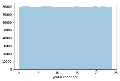
# histogram of years of experience
sns.distplot(data.yearsExperience, kde= False, bins=25)
<matplotlib.axes._subplots.AxesSubplot at 0x160243890>
# histogram of miles from metropolis
sns.distplot(data.milesFromMetropolis, kde = False)
<matplotlib.axes._subplots.AxesSubplot at 0x1600df690>
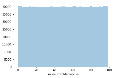
The data on years of experience and mile from metropolis seem reasonable. Both the mean and median years of experience required are about 12 years, with a min of 0 and a max of 24. Both the mean and the median number of miles from metropolis are about 50 miles, with a min of 0 and a max of 99. The values are almost evenly distributed across the range for both variables. Thus there seem to be no apparent outliers.
target.describe()
| salary | |
|---|---|
| count | 1000000.000000 |
| mean | 116.061818 |
| std | 38.717936 |
| min | 0.000000 |
| 25% | 88.000000 |
| 50% | 114.000000 |
| 75% | 141.000000 |
| max | 301.000000 |
# count the number of 0s
print('The number of 0s in salary: '+ str( sum(target.salary == 0)))
print('The minimum non-zero salary: ' + str(min(target.salary[target.salary != 0])))
The number of 0s in salary: 5
The minimum non-zero salary: 17
We can see that the target, salary, is relatively normally distributed, a bit positively skewed. Except for 5 zero salary, the rest are well above 0. These 5 may be outliers. Let’s remove them for now.
# remove zero-salary observations
zero_index = target[target.salary == 0].index
train.drop(zero_index, inplace=True)
target.drop(zero_index, inplace=True)

# update data
data = pd.concat([train, test], keys=['train','test'])
# describe the new data
target.describe()
| salary | |
|---|---|
| count | 999995.000000 |
| mean | 116.062398 |
| std | 38.717163 |
| min | 17.000000 |
| 25% | 88.000000 |
| 50% | 114.000000 |
| 75% | 141.000000 |
| max | 301.000000 |
data.select_dtypes(include=['object']).describe()
| jobId | companyId | jobType | degree | major | industry | |
|---|---|---|---|---|---|---|
| count | 1999995 | 1999995 | 1999995 | 1999995 | 1999995 | 1999995 |
| unique | 1999995 | 63 | 8 | 5 | 9 | 7 |
| top | JOB1362685306512 | COMP39 | SENIOR | HIGH_SCHOOL | NONE | WEB |
| freq | 1 | 32197 | 251088 | 475230 | 1066421 | 286217 |
# plot the distribution of the target
sns.distplot(target.salary)
<matplotlib.axes._subplots.AxesSubplot at 0x162acec10>
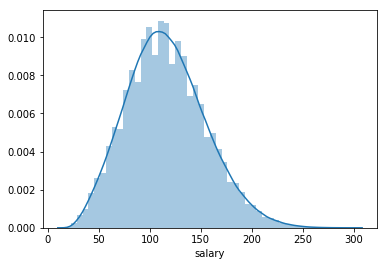
The description of categorical values shows that we are working with a fairly clean dataset. Of all the jobs posts included, there are only 63 companies, 8 job types, 9 majors, and 7 industries involoved. The jobs are fairly evenly distributed across companies, industry, degree, and job type. The only exception is major, with a lot of jobs not specifying a required major. The outcome variable is relatively normally distributed, slightly positively skewed. Since the skewness is only slight, we’ll leave the outcome variable as it.
Categorical Levels Check
Here let’s check if the categorical variables share the same levels in train and test data. If there are category levels in train but missing in test or vice versa, then we’d need to add a dummy level to test (or train) data to ensure consistent train and test data for the model.
# get categorical variable names
cat_vars = train.select_dtypes(include=['object']).columns
for i in cat_vars:
    print('The variable ' + i + ' has the same levels in the train and the test dataset:')
    # check if the intersection of levels is the same set as in train data
    print(len ( set(train[i]).intersection( test[i] ) ) == len( set(train[i])) )
The variable jobId has the same levels in the train and the test dataset:
False
The variable companyId has the same levels in the train and the test dataset:
True
The variable jobType has the same levels in the train and the test dataset:
True
The variable degree has the same levels in the train and the test dataset:
True
The variable major has the same levels in the train and the test dataset:
True
The variable industry has the same levels in the train and the test dataset:
True
The output above showed that the levels of all categorical variables have consistent levels in the train and the test data, except jobId (which should be the case, in fact we expected no overlap between the two). This is good since now we don’t need to worry about adding extra dummy levels for either train or test data.
Summary
In summary, we observed the following from the sanity checks:
- missing data - there are no missing values in the data.
- duplicates - there are no duplicates in the data.
- observation and feature order - the observations and features appear in the same order in the train, test, and target data.
- outliers - there are no apparent outliers in the data, 5 observations with a salary of 0 were removed. We’ll also look for outliders during the exploratory analysis.
- categorical levels - the train and test data have the same factor levels.
Descriptive Analysis
In this section, let’s analyze the correlation among the predictors and also between the predictors and the outcome. One nice way to present the correlations is to use a correlation matrix, such as the one that’s provided by the pairplot function in seaborn. The challenge is that this function does not support categorical variables, but we have quite a few categorical predictors. Let’s map the categorical levels to integers by converting them to factors.
# first, for visualization purpose, create numeric representation for categorical variables
train_cp = train.copy()
for i in train_cp.select_dtypes(include=['object']).columns.values:
    train_cp[i] = pd.factorize(train_cp[i])[0]
# add in the outcome var - salary
train_cp['salary'] = target.salary
# remove job Id
train_cp.drop(['jobId'],axis=1, inplace=True)
# second, Create a pair grid instance
# since the plot with all the train data took very long to generate
# let's plot on a random subset of the data
grid = sns.PairGrid(data= train_cp.sample(frac= 0.1) )

# Map the plots to the locations
grid = grid.map_offdiag(sns.regplot, marker = '+', x_jitter=.1, y_jitter=0.1)
grid = grid.map_diag(sns.distplot, kde = False)
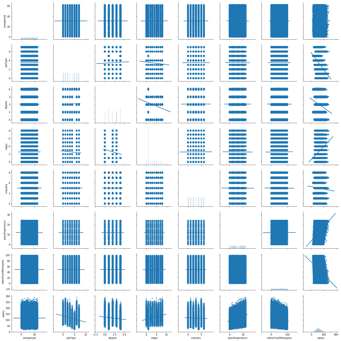
From the plots above, we can see that the data is fairly evenly distributed across the category levels for both categorical and numeric features. The only exception is the major feature, where the NONE level is very frequent.
As to the relationship between the outcome and the features, we have the following observations:
- In general, salary is higher for more experience, and for positions closer to metropolis. But there is a wide range of salary for each experience level and distance level. Also there are some notable outliers way above the average for each level.
- There are differences in salary across degrees, majors, industries, and job types, but not across companies. Similar to the relationship with numeric features, there is a wide range of salary for each level of the categorical features, maybe except for the JANITOR job type. Also there are some notable outliers way above the average for almost every level.
In the interest of space, I will not show individual bar plots, but we can learn a few of observations that are quite intuitive:
- There is no apparent association between degree and salary, except that no-specific major means less money.
- Job type matters. The C-suite position makes way more than the rest job types.
- Finance, oil, and web are some of the highest-paid industries, while service and education are paid the least.
Predictive Model
In this section, let’s predict salary using penalized linear models as a starting point.
We have 5 categorical features, and a goal to not only build a model, but also to estimate the feature contributions. With scikit-learn, we’d need to one-hot encode these features, which means that the contribution information for each categorical feature would be dispersed into individual variables for each level. To circumvent this issue, let’s use the h2o package, which encodes categorical features as factors and retains the level contributions to the single categorical feature.
import h2o
h2o.init()
Checking whether there is an H2O instance running at http://localhost:54321. connected.
| H2O cluster uptime: | 1 day 2 hours 16 mins |
| H2O cluster timezone: | America/Chicago |
| H2O data parsing timezone: | UTC |
| H2O cluster version: | 3.22.1.6 |
| H2O cluster version age: | 22 days |
| H2O cluster name: | H2O_from_python_mshen_n00a2o |
| H2O cluster total nodes: | 1 |
| H2O cluster free memory: | 2.624 Gb |
| H2O cluster total cores: | 8 |
| H2O cluster allowed cores: | 8 |
| H2O cluster status: | locked, healthy |
| H2O connection url: | http://localhost:54321 |
| H2O connection proxy: | None |
| H2O internal security: | False |
| H2O API Extensions: | Amazon S3, XGBoost, Algos, AutoML, Core V3, Core V4 |
| Python version: | 2.7.14 final |
# convert pandas DataFrame to H2OFrame
dat = train.merge(target, on = 'jobId')
df = h2o.H2OFrame(dat)
# split the data into train and test
splits = df.split_frame(ratios=[0.8], seed=42)
dtrain = splits[0]
dtest = splits[1]
Parse progress: |█████████████████████████████████████████████████████████| 100%
y = 'salary'
x = list(df.columns)
x.remove(y)  #remove the response
x.remove('jobId')
# The companyId feature doesn't seem to relate with salary, which comfirms our intuition.
# Also in production, there's always the possibility of predicting on unseen companies before.
# Therefore, let's remove the companyId feature for now
x.remove('companyId')
Linear Model
## grid search for best params with cross validation
from h2o.grid.grid_search import H2OGridSearch
from h2o.estimators.glm import H2OGeneralizedLinearEstimator
# grid search criteria, in the interest of time, let's set an upper limit to the runtime and max models
gs_criteria = {'strategy': 'RandomDiscrete',
              'max_models': 100,
              'max_runtime_secs': 6000,
              'stopping_metric': 'mae',
              'stopping_tolerance': 3,
              'seed': 1234,
              'stopping_rounds': 15}

# linear model parameter space
lm_params = {'alpha': [0.1, 0.5, 0.9],
             'lambda': [1e-4, 1e-2, 1e0, 1e2, 1e4]}

lm_gs = H2OGridSearch(model = H2OGeneralizedLinearEstimator(nfolds = 5),
                      hyper_params = lm_params,
                     search_criteria = gs_criteria)
lm_gs.train(x=x,y=y, training_frame=dtrain)
# display model IDs, hyperparameters, and MSE
# lm_gs.show()
# Get the grid results, sorted by validation mae
lm_gs_perf = lm_gs.get_grid(sort_by='mae', decreasing=True)
lm_gs_perf

# extract the top lm model, chosen by validation mae
lm_best = lm_gs.models[0]

# Now let's evaluate the model performance on a test set
# so we get an honest estimate of top model performance
lm_best_perf = lm_best.model_performance(dtest)

print('The best test MAE is %.2f' % lm_best_perf.mae())
print('The best test RMSE is %.2f' % lm_best_perf.rmse())
print('The best test R2 is %.2f' % lm_best_perf.r2())
The best test MAE is 15.85
The best test RMSE is 19.62
The best test R2 is 0.75
# get coef
coef = lm_best.coef()
# plot feature importance
coef_df = pd.DataFrame({'feature':coef.keys(), 'coefficient':coef.values()})

coef_df.reindex(coef_df.coefficient.abs().sort_values(ascending = False).index)
| coefficient | feature | |
|---|---|---|
| 12 | 115.651554 | Intercept |
| 17 | -34.583555 | jobType.JANITOR |
| 8 | 27.669385 | jobType.CEO |
| 15 | -22.043900 | jobType.JUNIOR |
| 16 | 17.929292 | jobType.CFO |
| 28 | 17.925786 | jobType.CTO |
| 2 | -16.191104 | industry.EDUCATION |
| 24 | 15.031780 | industry.OIL |
| 14 | 14.869542 | industry.FINANCE |
| 23 | -12.049542 | jobType.SENIOR |
| 19 | -11.159391 | industry.SERVICE |
| 25 | 10.121587 | degree.DOCTORAL |
| 21 | -9.430685 | degree.NONE |
| 3 | 8.327428 | major.ENGINEERING |
| 30 | 7.794749 | jobType.VICE_PRESIDENT |
| 1 | -7.222763 | major.NONE |
| 26 | -6.227290 | industry.AUTO |
| 11 | -5.954474 | major.LITERATURE |
| 29 | 5.882962 | industry.WEB |
| 27 | -5.747840 | degree.HIGH_SCHOOL |
| 5 | 5.334937 | major.BUSINESS |
| 13 | 5.005238 | degree.MASTERS |
| 6 | 2.846280 | major.MATH |
| 9 | -2.329465 | major.BIOLOGY |
| 22 | -2.145721 | jobType.MANAGER |
| 18 | 2.009992 | yearsExperience |
| 10 | 1.619933 | major.COMPSCI |
| 7 | -1.268621 | major.CHEMISTRY |
| 20 | -0.399243 | milesFromMetropolis |
| 31 | 0.000000 | major.PHYSICS |
| 4 | 0.000000 | degree.BACHELORS |
| 0 | 0.000000 | industry.HEALTH |
Random Forest Model
# now let's use the random forest algorithm to see if we can improve the performance
# import
from h2o.estimators.random_forest import H2ORandomForestEstimator
# rf parameters to be tuned
rf_params = {"ntrees" : [50,100],
              "max_depth" : [5,10],
              "sample_rate" : [0.3, 0.7],
              "mtries":[-1, 3, 7],
              "min_rows" : [3,5] }
# parameters for rf that don't need to be tuned
rf_p = {"seed": 42 ,
         "score_tree_interval": 3,
         "nfolds": 5}
# set up the grid
rf_gs = H2OGridSearch(model = H2ORandomForestEstimator(**rf_p),
                       hyper_params = rf_params,
                       search_criteria = gs_criteria)
# train the grid
rf_gs.train(x=x,y=y, training_frame=df)

# display model IDs, hyperparameters, and MSE
# rf_gs.show()
# Get the grid results, sorted by validation mae
rf_gs_perf = rf_gs.get_grid(sort_by='mae', decreasing=True)
rf_gs_perf

# extract the top lm model, chosen by validation mae
rf_best = rf_gs.models[0]

# Now let's evaluate the model performance on a test set
# so we get an honest estimate of top model performance
rf_best_perf = rf_best.model_performance(dtest)

print('The best test MAE is %.2f' % rf_best_perf.mae())
print('The best test RMSE is %.2f' % rf_best_perf.rmse())
print('The best test R2 is %.2f' % rf_best_perf.r2())
The best test MAE is 15.69
The best test RMSE is 19.44
The best test R2 is 0.75
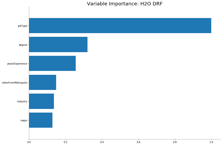
# plot feature importance
rf_best.varimp_plot()
Output Export
# write output
# convert test data to h2o frame
test_h2o = h2o.H2OFrame(test)
# determine the best model based on mae and use it for prediction
if rf_best_perf.mae() < lm_best_perf.mae():
    pred = rf_best.predict(test_h2o)
else:
    pred = lm_best.predict(test_h2o)
Parse progress: |█████████████████████████████████████████████████████████| 100%
drf prediction progress: |████████████████████████████████████████████████| 100%
# examine the basic stats of the salary predictions
pred.describe()
Rows:1000000
Cols:1
| predict | |
|---|---|
| type | real |
| mins | 29.2754525948 |
| mean | 116.050909815 |
| maxs | 216.278178101 |
| sigma | 32.3859060281 |
| zeros | 0 |
| missing | 0 |
| 0 | 106.993746109 |
| 1 | 100.914067307 |
| 2 | 170.002967072 |
| 3 | 108.953849945 |
| 4 | 111.065993118 |
| 5 | 149.859150085 |
| 6 | 96.3085207367 |
| 7 | 120.059133606 |
| 8 | 104.54789505 |
| 9 | 102.726793747 |
# concat jobId and salary prediction
out = test_h2o['jobId'].concat(pred)
# change names
out.set_names(list(target.columns))
# write the test output to a csv file
h2o.export_file(out, path = "test_salaries.csv")
Export File progress: |███████████████████████████████████████████████████| 100%
Conclusions and Suggestions
- In data exploration, we can observe that this dataset is quite clean and evenly distributed across levels, with only 5 0-salary observations.
- To predict the salary outcome, I built both a regularized linear model and a random forest model using the h2o package. The random forest model performed slightly better but took much longer to tune.
- Future directions - prediction explanations: If the rationale behind individual predictions is of interest, we can use the LIME method. LIME stands for Local Interpretable Model-Agnostic Explanations. Essentially, we attempt to understand why a model would make a certain prediction by building a locally-weighted linear model to approximate local predictions. Another viable approach is the SHAP values, which uses game theory to explain the contributions of each features to both individual and the overall predictions.